Geometry Representations

Surface Parameterization

A surface in Creo contains data that describes the boundary of the surface, and a pointer to the primitive surface on which it lies. The primitive surface is a three-dimensional geometric surface parameterized by two variables (u and v). The surface boundary consists of closed loops (contours) of edges. Each edge is attached to two surfaces, and each edge contains the u and v values of the portion of the boundary that it forms for both surfaces. Surface boundaries are traversed clockwise around the outside of a surface, so an edge has a direction in each surface with respect to the direction of traversal.

This section describes the surface parameterization. The surfaces are listed in order of complexity. For ease of use, the alphabetical listing of the data structures is as follows:

•

Cone

•

Coons Patch

•

Cylinder

•

Cylindrical Spline Surface

•

Fillet Surface

•

General Surface of Revolution

•

•

•

•

•

•

Plane

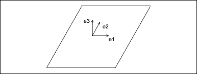
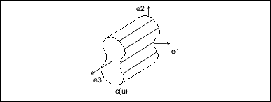
The plane entity consists of two perpendicular unit vectors (e1 and e2), the normal to the plane (e3), and the origin of the plane.

Data Format:

e1[3]       Unit vector, in the u direction
e2[3]       Unit vector, in the v direction
e3[3]       Normal to the plane
origin[3]   Origin of the plane

Parameterization:

(x, y, z) = u * e1 + v * e2 + origin

Cylinder

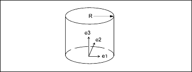
The generating curve of a cylinder is a line, parallel to the axis, at a distance R from the axis. The radial distance of a point is constant, and the height of the point is v.

Data Format:

e1[3]       Unit vector, in the u direction
e2[3]       Unit vector, in the v direction
e3[3]       Normal to the plane
origin[3]   Origin of the cylinder
radius      Radius of the cylinder

Parameterization:

(x, y, z) = radius * [cos(u) * e1 + sin(u) * e2] +
           v * e3 + origin

Engineering Notes:

For the cylinder, cone, torus, and general surface of revolution, a local coordinate system is used that consists of three orthogonal unit vectors (e1, e2, and e3) and an origin. The curve lies in the plane of e1 and e3, and is rotated in the direction from e1 to e2. The u surface parameter determines the angle of rotation, and the v parameter determines the position of the point on the generating curve.

Cone

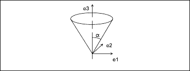
The generating curve of a cone is a line at an angle alpha to the axis of revolution that intersects the axis at the origin. The v parameter is the height of the point along the axis, and the radial distance of the point is v * tan(alpha).

Data Format:

e1[3]      Unit vector, in the u direction
e2[3]      Unit vector, in the v direction
e3[3]      Normal to the plane
origin[3]  Origin of the cone
alpha      Angle between the axis of the cone 
           and the generating line

Parameterization:

(x, y, z) = v * tan(alpha) * [cos(u) * e1 + 
            sin(u) * e2] + v * e3 + origin

Torus

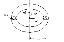
The generating curve of a torus is an arc of radius R2 with its center at a distance R1 from the origin. The starting point of the generating arc is located at a distance R1 + R2 from the origin, in the direction of the first vector of the local coordinate system. The radial distance of a point on the torus is R1 + R2 * cos(v), and the height of the point along the axis of revolution is R2 * sin(v).

Data Format:

e1[3]      Unit vector, in the u direction
e2[3]      Unit vector, in the v direction
e3[3]      Normal to the plane
origin[3]  Origin of the torus
radius1    Distance from the center of the 
           generating arc to the axis of 
           revolution
radius2    Radius of the generating arc

Parameterization:

(x, y, z) = (R1 + R2 * cos(v)) * [cos(u) * e1 + 
            sin(u) * e2] + R2 * sin(v) * e3 + 
            origin

General Surface of Revolution

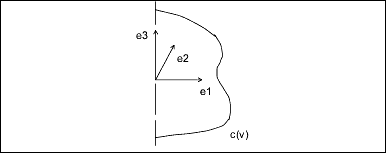
A general surface of revolution is created by rotating a curve entity, usually a spline, around an axis. The curve is evaluated at the normalized parameter v, and the resulting point is rotated around the axis through an angle u. The surface of revolution data structure consists of a local coordinate system and a curve structure.

Data Format:

e1[3]       Unit vector, in the u direction
e2[3]       Unit vector, in the v direction
e3[3]       Normal to the plane
origin[3]   Origin of the surface of revolution
curve       Generating curve

Parameterization:

curve(v) = (c1, c2, c3) is a point on the curve.

(x, y, z) = [c1 * cos(u) - c2 * sin(u)] * e1 + 
            [c1 * sin(u) + c2 * cos(u)] * e2 + 
            c3 * e3 + origin

Ruled Surface

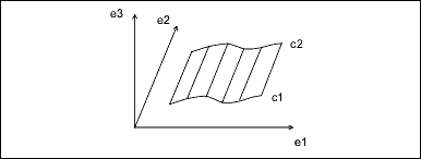
A ruled surface is the surface generated by interpolating linearly between corresponding points of two curve entities. The u coordinate is the normalized parameter at which both curves are evaluated, and the v coordinate is the linear parameter between the two points. The curves are not defined in the local coordinate system of the part, so the resulting point must be transformed by the local coordinate system of the surface.

Data Format:

e1[3]      Unit vector, in the u direction
e2[3]      Unit vector, in the v direction
e3[3]      Normal to the plane
origin[3]  Origin of the ruled surface
curve_1    First generating curve
curve_2    Second generating curve

Parameterization:

(x', y', z') is the point in local coordinates.
(x', y', z') = (1 - v) * C1(u) + v * C2(u)
(x, y, z) = x' * e1 + y' * e2 + z' * e3 + origin

Tabulated Cylinder

A tabulated cylinder is calculated by projecting a curve linearly through space. The curve is evaluated at the u parameter, and the z coordinate is offset by the v parameter. The resulting point is expressed in local coordinates and must be transformed by the local coordinate system to be expressed in part coordinates.

Data Format:

e1[3]      Unit vector, in the u direction
e2[3]      Unit vector, in the v direction
e3[3]      Normal to the plane
origin[3]  Origin of the tabulated cylinder
curve      Generating curve

Parameterization:

(x', y', z') is the point in local coordinates.
(x', y', z') = C(u) + (0, 0, v)
(x, y, z) = x' * e1 + y' * e2 + z' * e3 + origin

Coons Patch

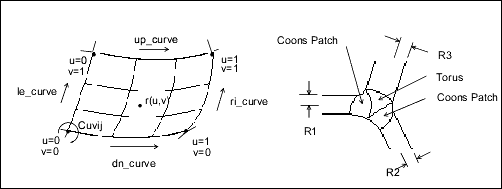
A Coons patch is used to blend surfaces together. For example, you would use a Coons patch at a corner where three fillets (each of a different radius) meet.

Data Format:

le_curve               u = 0 boundary
ri_curve               u = 1 boundary
dn_curve               v = 0 boundary
up_curve               v = 1 boundary
point_matrix[2][2]     Corner points
uvder_matrix[2][2]     Corner mixed derivatives

Fillet Surface

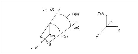
A fillet surface is found where a round or a fillet is placed on a curved edge, or on an edge with non-constant arc radii. On a straight edge, a cylinder would be used to represent the fillet.

Data Format:

pnt_spline   P(v) spline running along the u = 0 boundary
ctr_spline   C(v) spline along the centers of the
             fillet arcs
tan_spline   T(v) spline of unit tangents to the
             axis of the fillet arcs

Parameterization:

R(v) = P(v) - C(v)
(x,y,z) = C(v) + R(v) * cos(u) + T(v) X R(v) * 
          sin(u)

Spline Surface

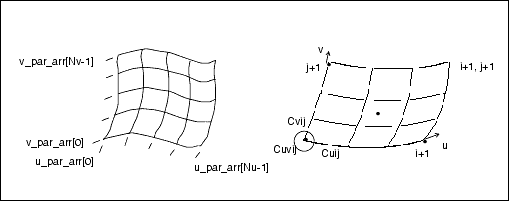
The parametric spline surface is a nonuniform bicubic spline surface that passes through a grid with tangent vectors given at each point. The grid is curvilinear in uv space. Use this for bicubic blending between corner points.

Data Format:

u_par_arr[]     Point parameters, in the u
                direction, of size Nu
v_par_arr[]     Point parameters, in the v
                direction, of size Nv
point_arr[][3]  Array of interpolant points, of
                size Nu x Nv
u_tan_arr[][3]  Array of u tangent vectors
                at interpolant points, of size
                Nu x Nv
v_tan_arr[][3]  Array of v tangent vectors at
                interpolant points, of size
                Nu x Nv
uvder_arr[][3]  Array of mixed derivatives at
                interpolant points, of size
                Nu x Nv

Engineering Notes:

•

Allows for a unique 3x3 polynomial around every patch.

•

There is second order continuity across patch boundaries.

•

The point and tangent vectors represent the ordering of an array of [i][j], where u varies with j, and v varies with j. In walking through the point_arr[][3], you will find that the innermost variable representing v(j) varies first.

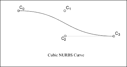
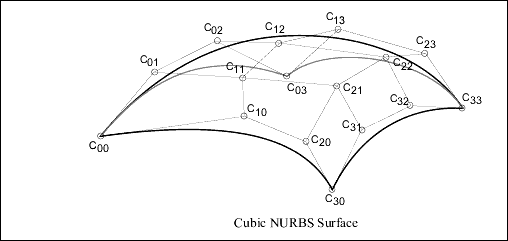
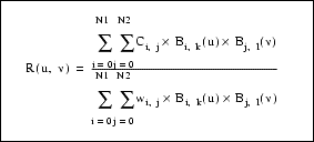
NURBS Surface

The NURBS surface is defined by basis functions (in u and v), expandable arrays of knots, weights, and control points.

Data Format:

deg[2]             Degree of the basis
                   functions (in u and v)
u_par_arr[]        Array of knots on the 
                   parameter line u
v_par_arr[]        Array of knots on the
                   parameter line v
wghts[]            Array of weights for
                   rational NURBS, otherwise
                   NULL
c_point_arr[][3]   Array of control points

Definition:

k   = degree in u
l   = degree in v
N1  = (number of knots in u) - (degree in u) - 2
N2  = (number of knots in v) - (degree in v) - 2
Bi,k = basis function in u
Bj, l  = basis function in v
wij  = weights
Ci, j   = control points (x,y,z) * wi,j

Engineering Notes:

The weights and c_points_arr arrays represent matrices of size wghts[N1+1] [N2+1] and c_points_arr [N1+1] [N2+1]. Elements of the matrices are packed into arrays in row-major order.

Cylindrical Spline Surface

The cylindrical spline surface is a nonuniform bicubic spline surface that passes through a grid with tangent vectors given at each point. The grid is curvilinear in modeling space.

Data Format:

e1[3]      x' vector of the local coordinate
           system
e2[3]      y' vector of the local coordinate
           system
e3[3]      z' vector of the local coordinate
           system, which corresponds to the
           axis of revolution of the surface
origin[3]  Origin of the local coordinate
           system
splsrf     Spline surface data structure

The spline surface data structure contains the following fields:

u_par_arr[]         Point parameters, in the
                    u direction, of size Nu
v_par_arr[]         Point parameters, in the
                    v direction, of size Nv
point_arr[][3]      Array of points, in 
                    cylindrical coordinates,
                    of size Nu x Nv. The array
                    components are as follows:
                        point_arr[i][0] - Radius
                        point_arr[i][1] - Theta
                        point_arr[i][2] - Z
u_tan_arr[][3]      Array of u tangent vectors.
                    in cylindrical coordinates,
                    of size Nu x Nv
v_tan_arr[][3]      Array of v tangent vectors,
                    in cylindrical coordinates,
                    of size Nu x Nv
uvder_arr[][3]      Array of mixed derivatives,
                    in cylindrical coordinates,
                    of size Nu x Nv

Engineering Notes:

If the surface is represented in cylindrical coordinates (r, theta, z), the local coordinate system values (x',y', z') are interpreted as follows:

x' = r cos (theta)
y' = r sin (theta)
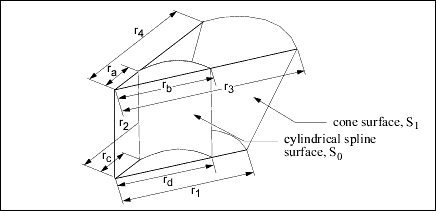
z' = z

A cylindrical spline surface can be obtained, for example, by creating a smooth rotational blend (shown in the figure).

In some cases, you can replace a cylindrical spline surface with a surface such as a plane, cylinder, or cone. For example, in the figure, the cylindrical spline surface S1 was replaced with a cone (r1 = r2, r3 = r4, and r1 ≠ r3).

If a replacement cannot be done (such as for the surface S0 in the figure (ra ≠ rb or rc ≠ rd)), leave it as a cylindrical spline surface representation.

Edge and Curve Parameterization

This parameterization represents edges (line, arc, and spline) as well as the curves (line, arc, spline, and NURBS) within the surfaces.

This section describes edges and curves, arranged in order of complexity. For ease of use, the alphabetical listing is as follows:

•

•

•

•

Line

Data Format:

end1[3]   Starting point of the line
end2[3]   Ending point of the line

Parameterization:

(x, y, z) = (1 - t) * end1 + t * end2

Arc

The arc entity is defined by a plane in which the arc lies. The arc is centered at the origin, and is parameterized by the angle of rotation from the first plane unit vector in the direction of the second plane vector. The start and end angle parameters of the arc and the radius are also given. The direction of the arc is counterclockwise if the start angle is less than the end angle, otherwise it is clockwise.

Data Format:

vector1[3]    First vector that defines the
              plane of the arc
vector2[3]    Second vector that defines the
              plane of the arc
origin[3]     Origin that defines the plane
              of the arc
start_angle   Angular parameter of the starting
              point
end_angle     Angular parameter of the ending
              point
radius        Radius of the arc.

Parameterization:

t' (the unnormalized parameter) is 
   (1 - t) * start_angle + t * end_angle
(x, y, z) = radius * [cos(t') * vector1 +
   sin(t') * vector2] + origin

Spline

The spline curve entity is a nonuniform cubic spline, defined by a series of three-dimensional points, tangent vectors at each point, and an array of unnormalized spline parameters at each point.

Data Format:

par_arr[]     Array of spline parameters
              (t) at each point.
pnt_arr[][3]  Array of spline interpolant points
tan_arr[][3]  Array of tangent vectors at
              each point

Parameterization:

x, y, and z are a series of unique cubic functions, one per segment, fully determined by the starting and ending points, and tangents of each segment.

Let p_max be the parameter of the last spline point. Then, t, the unnormalized parameter, is t * p_max.

Locate the ith spline segment such that:

par_arr[i] < t' < par_arr[i+1]

(If t < 0 or t > +1, use the first or last segment.)

t0 = (t' - par_arr[i])   / (par_arr[i+1] - par_arr[i])
t1 = (par_arr[i+1] - t') / (par_arr[i+1] - par_arr[i])

NURBS

The NURBS (nonuniform rational B-spline) curve is defined by expandable arrays of knots, weights, and control points.

Data Format:

degree        Degree of the basis function
params[]      Array of knots
weights[]     Array of weights for rational 
              NURBS, otherwise NULL.
c_pnts[][3]   Array of control points

Definition:

k     = degree of basis function
N    = (number of knots) - (degree) - 2
wi   = weights
Ci    = control points (x, y, z) * wi
Bi,k = basis functions

By this equation, the number of control points equals N+1.

References:

Faux, I.D., M.J. Pratt. Computational Geometry for Design and Manufacture. Ellis Harwood Publishers, 1983.

Mortenson, M.E. Geometric Modeling. John Wiley & Sons, 1985.